40 excel chart custom data labels
How to Add Data Labels to Scatter Plot in Excel (2 Easy Ways) - ExcelDemy At first, go to the sheet Chart Elements. Then, select the Scatter Plot already inserted. After that, go to the Chart Design tab. Later, select Add Chart Element > Data Labels > None. This is how we can remove the data labels. Read More: Use Scatter Chart in Excel to Find Relationships between Two Data Series. 2. Add Custom Labels to x-y Scatter plot in Excel Step 1: Select the Data, INSERT -> Recommended Charts -> Scatter chart (3 rd chart will be scatter chart) Let the plotted scatter chart be Step 2: Click the + symbol and add data labels by clicking it as shown below Step 3: Now we need to add the flavor names to the label.Now right click on the label and click format data labels. Under LABEL OPTIONS select Value From …
DataLabels object (Excel) | Microsoft Learn The following example sets the number format for data labels on series one on chart sheet one. With Charts(1).SeriesCollection(1) .HasDataLabels = True .DataLabels.NumberFormat = "##.##" End With Use DataLabels (index), where index is the data-label index number, to return a single DataLabel object. The following example sets the number format ...
Excel chart custom data labels
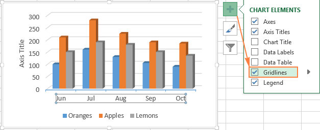
Data Labels in Excel Pivot Chart (Detailed Analysis) 7 Suitable Examples with Data Labels in Excel Pivot Chart Considering All Factors 1. Adding Data Labels in Pivot Chart 2. Set Cell Values as Data Labels 3. Showing Percentages as Data Labels 4. Changing Appearance of Pivot Chart Labels 5. Changing Background of Data Labels 6. Dynamic Pivot Chart Data Labels with Slicers 7. Use Excel with earlier versions of Excel - support.microsoft.com A chart contains a title or data label with more than 255 characters. Characters beyond the 255-character limit will not be saved. What it means Chart or axis titles and data labels are limited to 255 characters in Excel 97-2003, and any characters beyond this limit will be lost. Label Specific Excel Chart Axis Dates • My Online Training Hub Jul 09, 2020 · Step 5 – Add Data Labels to the 'Date Label Position' Series. Use the drop-down list on the Chart Format tab to select the ‘date label position’ series as it’s no longer visible in the chart. While you’re adding elements (4 in image below) also remove the gridlines and legend if required (6 & 7 in image below): ... Custom Excel Chart ...
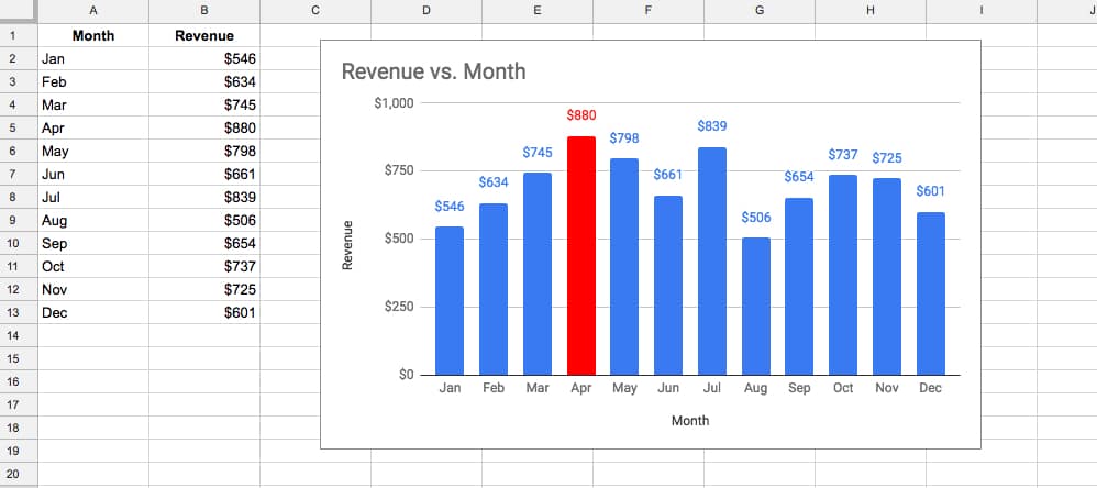
Excel chart custom data labels. Custom data labels in a chart - Get Digital Help You can easily change data labels in a chart. Select a single data label and enter a reference to a cell in the formula bar. You can also edit data labels, one by one, on the chart. With many data labels, the task becomes quickly boring and time-consuming. But wait, there is a third option using a duplicate series on a secondary axis. The ... Edit titles or data labels in a chart - support.microsoft.com The first click selects the data labels for the whole data series, and the second click selects the individual data label. Right-click the data label, and then click Format Data Label or Format Data Labels. Click Label Options if it's not selected, and then select the Reset Label Text check box. Top of Page How to create Custom Data Labels in Excel Charts - Efficiency 365 Create the chart as usual Add default data labels Click on each unwanted label (using slow double click) and delete it Select each item where you want the custom label one at a time Press F2 to move focus to the Formula editing box Type the equal to sign Now click on the cell which contains the appropriate label Press ENTER That's it. Custom Chart Data Labels In Excel With Formulas - How To Excel At Excel Follow the steps below to create the custom data labels. Select the chart label you want to change. In the formula-bar hit = (equals), select the cell reference containing your chart label's data. In this case, the first label is in cell E2. Finally, repeat for all your chart laebls.
Excel Custom Chart Labels • My Online Training Hub Note: Excel 2013 onward also requires this step if you have more than one series you want to position your labels above. Step 1: Select cells A26:D38 and insert a column Chart. Step 2: Select the Max series and plot it on the Secondary Axis: double click the Max series > Format Data Series > Secondary Axis: Step 3: Insert labels on the Max ... › 509290 › how-to-use-cell-valuesHow to Use Cell Values for Excel Chart Labels - How-To Geek Mar 12, 2020 · Select the chart, choose the “Chart Elements” option, click the “Data Labels” arrow, and then “More Options.” Uncheck the “Value” box and check the “Value From Cells” box. Select cells C2:C6 to use for the data label range and then click the “OK” button. › 07 › 25How to create waterfall chart in Excel - Ablebits.com Jul 25, 2014 · However, when you refer to the data table, you'll see that the represented values are different. For more accurate analysis I'd recommend to add data labels to the columns. Select the series that you want to label. Right-click and choose the Add Data Labels option from the context menu. Repeat the process for the other series. Custom Data Labels with Colors and Symbols in Excel Charts - [How To ... The basic idea behind custom label is to connect each data label to certain cell in the Excel worksheet and so whatever goes in that cell will appear on the chart as data label. So once a data label is connected to a cell, we apply custom number formatting on the cell and the results will show up on chart also.
peltiertech.com › broken-y-axis-inBroken Y Axis in an Excel Chart - Peltier Tech Nov 18, 2011 · – For the axis, you could hide the missing label by leaving the corresponding cell blank if it’s a line or bar chart, or by using a custom number format like [<2010]0;[>2010]0;;. You’ve explained the missing data in the text. No need to dwell on it in the chart. The gap in the data or axis labels indicate that there is missing data. Excel Charts: Creating Custom Data Labels - YouTube Excel Charts: Creating Custom Data Labels 91,765 views Jun 26, 2016 210 Dislike Share Save Mike Thomas 4.58K subscribers In this video I'll show you how to add data labels to a chart in Excel and... How to Use Cell Values for Excel Chart Labels - How-To Geek Mar 12, 2020 · Select the chart, choose the “Chart Elements” option, click the “Data Labels” arrow, and then “More Options.” Uncheck the “Value” box and check the “Value From Cells” box. Select cells C2:C6 to use for the data label range and then click the “OK” button. How to add data labels from different column in an Excel chart? Right click the data series in the chart, and select Add Data Labels > Add Data Labels from the context menu to add data labels. 2. Click any data label to select all data labels, and then click the specified data label to select it only in the chart. 3.
Add / Move Data Labels in Charts – Excel & Google Sheets ...
Using the CONCAT function to create custom data labels for an Excel chart Use the chart skittle (the "+" sign to the right of the chart) to select Data Labels and select More Options to display the Data Labels task pane. Check the Value From Cells checkbox and select the cells containing the custom labels, cells C5 to C16 in this example.

Adding rich data labels to charts in Excel 2013 | Microsoft ...
support.microsoft.com › en-us › officeUse Excel with earlier versions of Excel - support.microsoft.com A chart contains a title or data label with more than 255 characters. Characters beyond the 255-character limit will not be saved. What it means Chart or axis titles and data labels are limited to 255 characters in Excel 97-2003, and any characters beyond this limit will be lost.

Custom Chart Data Labels Pic 5 - Excel Dashboard Templates
How To Add Data Labels In Excel - newall.northminster.info Add custom data labels from the column "x axis labels". In this second method, we will add the x and y axis labels in excel by chart element button. Source: . Click add chart element chart elements button > data labels in the upper. Right click the data series in the chart, and select add data labels > add. Source: superuser.com

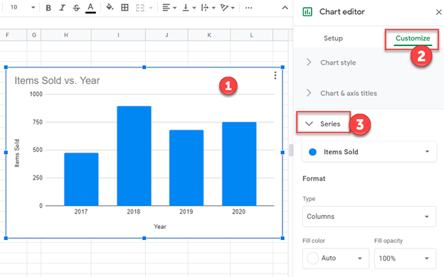
Google Workspace Updates: New chart text and number ...
Add or remove data labels in a chart - support.microsoft.com Click the data series or chart. To label one data point, after clicking the series, click that data point. In the upper right corner, next to the chart, click Add Chart Element > Data Labels. To change the location, click the arrow, and choose an option. If you want to show your data label inside a text bubble shape, click Data Callout.
Excel Charts: Creating Custom Data Labels
How to add text labels on Excel scatter chart axis - Data Cornering Add dummy series to the scatter plot and add data labels. 4. Select recently added labels and press Ctrl + 1 to edit them. Add custom data labels from the column "X axis labels". Use "Values from Cells" like in this other post and remove values related to the actual dummy series. Change the label position below data points.

Change axis labels in a chart
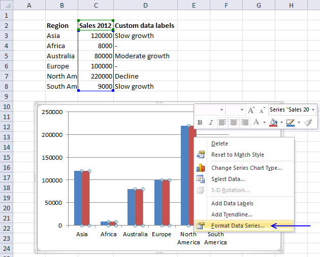
How to Change Excel Chart Data Labels to Custom Values? - Chandoo.org May 05, 2010 · Now, click on any data label. This will select “all” data labels. Now click once again. At this point excel will select only one data label. Go to Formula bar, press = and point to the cell where the data label for that chart data point is defined. Repeat the process for all other data labels, one after another. See the screencast.

charts - How do I create custom axes in Excel? - Super User
chandoo.org › wp › change-data-labels-in-chartsHow to Change Excel Chart Data Labels to Custom Values? May 05, 2010 · Now, click on any data label. This will select “all” data labels. Now click once again. At this point excel will select only one data label. Go to Formula bar, press = and point to the cell where the data label for that chart data point is defined. Repeat the process for all other data labels, one after another. See the screencast.
How to Change Horizontal Axis Labels in Excel 2010 - Solve ...
Apply Custom Data Labels to Charted Points - Peltier Tech There are a number of ways to apply custom data labels to your chart: Manually Type Desired Text for Each Label Manually Link Each Label to Cell with Desired Text Use the Chart Labeler Program Use Values from Cells (Excel 2013 and later) Write Your Own VBA Routines Manually Type Desired Text for Each Label
How can I format individual data points in Google Sheets ...
› label-specific-excelLabel Specific Excel Chart Axis Dates • My Online Training Hub Jul 09, 2020 · Note: if your chart has negative values then set the ‘Date Label Position’ to a value lower than the minimum negative value so that the labels sit below the line in the chart. Step 1 - Insert a regular line or scatter chart. I’m going to insert a scatter chart so I can show you another trick most people don’t know*.
Excel charts: add title, customize chart axis, legend and ...
Example: Charts with Data Labels — XlsxWriter Documentation Chart 1 in the following example is a chart with standard data labels: Chart 6 is a chart with custom data labels referenced from worksheet cells: Chart 7 is a chart with a mix of custom and default labels. The None items will get the default value. We also set a font for the custom items as an extra example: Chart 8 is a chart with some ...
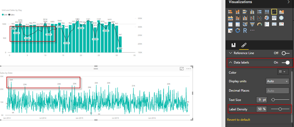
Solved: Data Labels - Microsoft Power BI Community
Excel Chart Vertical Axis Text Labels • My Online Training Hub Apr 14, 2015 · So all we need to do is get that bar chart into our line chart, align the labels to the line chart and then hide the bars. We’ll do this with a dummy series: Copy cells G4:H10 (note row 5 is intentionally blank) > CTRL+C to copy the cells > select the chart > CTRL+V to paste the dummy data into the chart.

How to set and format data labels for Excel charts in C#
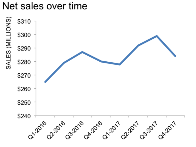
3 Types of Line Graph/Chart: + [Examples & Excel Tutorial] Apr 20, 2020 · Multiple data points indicate various statistics over time. The graph above, for instance, shows the population of a particular community over a period of time with the data points indicating the population size at a certain time. Data points can also be visualized using markers as opposed to dots. Labels
Custom data labels in a chart
How to Automatically Update Data in Another Sheet in Excel Linking data in a real data set is more complex and depends on your situation. You might need to use techniques other than those listed above. If you are in a rush and want your problem answered by an Excel expert, try our service. The experts are available to help you 24/7. The first question is free.

How to Create a Pie Chart in Excel | Smartsheet
Change the format of data labels in a chart To get there, after adding your data labels, select the data label to format, and then click Chart Elements > Data Labels > More Options. To go to the appropriate area, click one of the four icons ( Fill & Line, Effects, Size & Properties ( Layout & Properties in Outlook or Word), or Label Options) shown here.
Excel Data Labels: How to add totals as labels to a stacked ...
How to create waterfall chart in Excel - Ablebits.com Jul 25, 2014 · However, when you refer to the data table, you'll see that the represented values are different. For more accurate analysis I'd recommend to add data labels to the columns. Select the series that you want to label. Right-click and choose the Add Data Labels option from the context menu. Repeat the process for the other series.
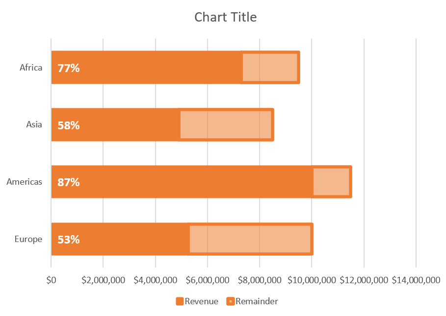
How to Create Progress Charts (Bar and Circle) in Excel ...
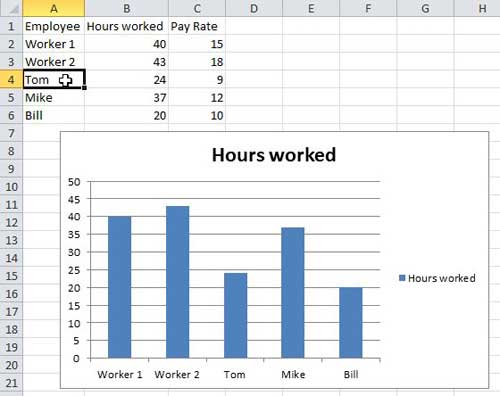
Make your Excel charts easier to read with custom data labels One way you can make your chart easier to read is to. remove the data series markers altogether and replace them with custom data. labels. For example, suppose you have the Months listed in A6:A17 ...

Apply Custom Data Labels to Charted Points - Peltier Tech
› add-custom-labelsAdd Custom Labels to x-y Scatter plot in Excel Step 1: Select the Data, INSERT -> Recommended Charts -> Scatter chart (3 rd chart will be scatter chart) Let the plotted scatter chart be Step 2: Click the + symbol and add data labels by clicking it as shown below. Step 3: Now we need to add the flavor names to the label. Now right click on the label and click format data labels.
Custom Chart Data Labels In Excel With Formulas
Broken Y Axis in an Excel Chart - Peltier Tech Nov 18, 2011 · – For the axis, you could hide the missing label by leaving the corresponding cell blank if it’s a line or bar chart, or by using a custom number format like [<2010]0;[>2010]0;;. You’ve explained the missing data in the text. No need to dwell on it in the chart. The gap in the data or axis labels indicate that there is missing data.

Change the format of data labels in a chart
Create Custom Data Labels. Excel Charting. - YouTube Are you looking to create custom data labels to your Excel chart? Maybe you want to add the title of a song or the name of a magazine. Whatever the reason, i...

How to Create a Pie Chart in Excel | Smartsheet
Label Specific Excel Chart Axis Dates • My Online Training Hub Jul 09, 2020 · Step 5 – Add Data Labels to the 'Date Label Position' Series. Use the drop-down list on the Chart Format tab to select the ‘date label position’ series as it’s no longer visible in the chart. While you’re adding elements (4 in image below) also remove the gridlines and legend if required (6 & 7 in image below): ... Custom Excel Chart ...

How to create Custom Data Labels in Excel Charts
Use Excel with earlier versions of Excel - support.microsoft.com A chart contains a title or data label with more than 255 characters. Characters beyond the 255-character limit will not be saved. What it means Chart or axis titles and data labels are limited to 255 characters in Excel 97-2003, and any characters beyond this limit will be lost.

Custom data labels in a chart
Data Labels in Excel Pivot Chart (Detailed Analysis) 7 Suitable Examples with Data Labels in Excel Pivot Chart Considering All Factors 1. Adding Data Labels in Pivot Chart 2. Set Cell Values as Data Labels 3. Showing Percentages as Data Labels 4. Changing Appearance of Pivot Chart Labels 5. Changing Background of Data Labels 6. Dynamic Pivot Chart Data Labels with Slicers 7.

Directly Labeling Your Line Graphs | Depict Data Studio
Custom Y-Axis Labels in Excel - PolicyViz

Display Customized Data Labels on Charts & Graphs

Adding rich data labels to charts in Excel 2013 | Microsoft ...

Custom Data Labels with Colors and Symbols in Excel Charts ...
Excel axis labels - supercategory — storytelling with data

Dynamic Number Format for Millions and Thousands - PK: An ...

Google Workspace Updates: Get more control over chart data ...

Change axis labels in a chart

Change the format of data labels in a chart

How to add axis labels in excel | WPS Office Academy

Custom data labels in a chart
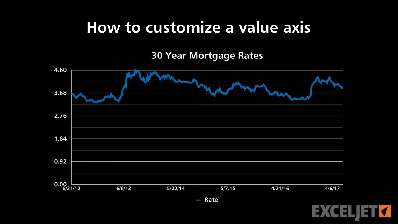
How to customize a value axis

How to Add Data Labels to your Excel Chart in Excel 2013

How to Add Axis Labels to a Chart in Excel | CustomGuide

How to Customize for a GREAT-Looking Excel Chart

Data Labels | FlexChart | ComponentOne

Adding rich data labels to charts in Excel 2013 | Microsoft ...
Post a Comment for "40 excel chart custom data labels"