41 how to create a scatter plot in excel with labels

Add vertical line to Excel chart: scatter plot, bar and line graph 15.05.2019 · Right-click anywhere in your scatter chart and choose Select Data… in the pop-up menu.; In the Select Data Source dialogue window, click the Add button under Legend Entries (Series):; In the Edit Series dialog box, do the following: . In the Series name box, type a name for the vertical line series, say Average.; In the Series X value box, select the independentx-value … How to display text labels in the X-axis of scatter chart in Excel? Display text labels in X-axis of scatter chart Actually, there is no way that can display text labels in the X-axis of scatter chart in Excel, but we can create a line chart and make it look like a scatter chart. 1. Select the data you use, and click Insert > Insert Line & Area Chart > Line with Markers to select a line chart. See screenshot: 2.

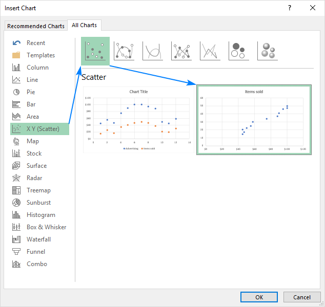
how to make a scatter plot in Excel — storytelling with data Select "Scatter" from the options in the "Recommended Charts" section of your ribbon. Excel will automatically create a scatter plot for you in the same sheet as your data, using the first column of your dataset as the horizontal (X) axis, and the second column as your vertical (Y) axis. A quick note here: in creating scatter plots, a ...

How to create a scatter plot in excel with labels

How to Make a Scatter Plot in Excel | GoSkills Create a scatter plot from the first data set by highlighting the data and using the Insert > Chart > Scatter sequence. In the above image, the Scatter with straight lines and markers was selected, but of course, any one will do. The scatter plot for your first series will be placed on the worksheet. Select the chart. How to Make a Scatter Plot in Excel and Present Your Data - MUO 17.05.2021 · When you create a scatter plot in Microsoft Excel, you have the freedom to customize almost every element of it. You can modify sections like axis titles, chart titles, chart colors, legends, and even hide the gridlines. If you want to reduce the plot area, follow these steps: Double-click on the horizontal (X) or vertical (Y) axis to open Format Axis. Under the Axis … How to Make a Scatter Plot in Excel to Present Your Data - groovyPost Select the data for your chart. If you have column headers that you want to include, you can select those as well. By default, the chart title will be the header for your y-axis column. But you ...

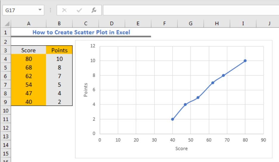
How to create a scatter plot in excel with labels. Scatter Plot Chart in Excel (Examples) | How To Create Scatter ... - EDUCBA Step 1: Select the data. Step 2: Go to Insert > Chart > Scatter Chart > Click on the first chart. Step 3: This will create the scatter diagram. Step 4: Add the axis titles, increase the size of the bubble and Change the chart title as we have discussed in the above example. Step 5: We can add a trend line to it. Creating Tables and Scatter Plots in Excel - Instructables Step 4: Highlight Table to Form a Scatter Plot. 4.1 Drag your mouse from one top corner of the table to the opposite bottom corner so that the entire table is highlighted. 4.2 Select the scatter plot among the chart options (see above image). Add Tip. How to find, highlight and label a data point in Excel scatter plot Select the Data Labels box and choose where to position the label. By default, Excel shows one numeric value for the label, y value in our case. To display both x and y values, right-click the label, click Format Data Labels…, select the X Value and Y value boxes, and set the Separator of your choosing: Label the data point by name Want To Know How to Create A Scatter Plot In Excel? Here's How ... Click on a point on the chart again to activate it, right-click to show the "Add Data Labels" option again, and then select "Add Data Labels" in the rollout menu. The numbers will appear and can be...

How to Create a Quadrant Chart in Excel – Automate Excel Step #1: Create an empty XY scatter chart. Why empty? Because as experience shows, Excel may simply leave out some of the values when you plot an XY scatter chart. Building the chart from scratch ensures that nothing gets lost along the way. Click on any empty cell. Switch to the Insert tab. Click the “Insert Scatter (X, Y) or Bubble Chart.” How to create a scatter plot in Excel with 3 variables Editing scatter plots Theres a lot of customization available to make your chart look better. The easiest way to do this is by clicking Chart Design on the tab list. (Dont forget to click on your chart first or else this tab wont show.) Then, hover over the different chart styles available. This will give a preview of the style on your chart. Creating Scatter Plot with Marker Labels - Microsoft Community Right click any data point and click 'Add data labels and Excel will pick one of the columns you used to create the chart. Right click one of these data labels and click 'Format data labels' and in the context menu that pops up select 'Value from cells' and select the column of names and click OK. Scatter plot excel with labels - kdfssh.mobiwiki.de Is it possible to put text labels on the X axis of a scatter plot ? Well, actually, I'm trying to use a bubble plot but the same issue applies. No matter how hard I try I cannot get the labels to come out as text labels . The labels are numeric but they should not be treated as numbers. energy assistance program. how to give a girl your number ...

How to create a Scatterplot with Dynamic Reference Lines in Excel 1. On the Developer tab, in the Controls group, click on the Insert icon and then select the Group Box (Form Control) from the Form Controls dropdown menu. 2. Next, with the mouse, draw a rectangle on the worksheet to insert the Group Box. 3. Free Scatter Plot Maker - Create Scatter Graphs Online | Visme Import data from Excel, customize labels and plot colors and export your design. Create easy-to-read scatter plots using our free scatter plot maker. Import data from Excel, customize labels and plot colors and export your design. Create Your Scatter Plot It’s free and easy to use. This website uses cookies to improve the user experience. By using our website you consent to all cookies … Microsoft Excel - Creating a Scatter Plot with trend line and axis labels A video demonstrating how to create a scatter plot, with title axis labels, and trend line on Microsoft Excel. (Also a little extra at the end on printing) Scatter Plot in Excel (In Easy Steps) - Excel Easy To create a scatter plot with straight lines, execute the following steps. 1. Select the range A1:D22. 2. On the Insert tab, in the Charts group, click the Scatter symbol. 3. Click Scatter with Straight Lines. Note: also see the subtype Scatter with Smooth Lines. Note: we added a horizontal and vertical axis title.

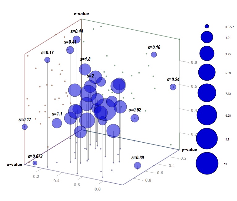
3d scatter plot for MS Excel

How to Create a Q-Q Plot in Excel - Statology Mar 27, 2020 · Example: Q-Q Plot in Excel. Perform the follow steps to create a Q-Q plot for a set of data. Step 1: Enter and sort the data. Enter the following data into one column: Note that this data is already sorted from smallest to largest. If your data is not already sorted, go to the Data tab along the top ribbon in Excel, then go to the Sort & Filter ...

How to Create a Scatter Plot in Excel

Use text as horizontal labels in Excel scatter plot Edit each data label individually, type a = character and click the cell that has the corresponding text. This process can be automated with the free XY Chart Labeler add-in. Excel 2013 and newer has the option to include "Value from cells" in the data label dialog. Format the data labels to your preferences and hide the original x axis labels.

Want to know how to create a scatter plot in Excel? Here’s our guide

X-Y Scatter Plot With Labels Excel for Mac This is standard functionality in Excel for the Mac as far as I know. Now, this picture does not show the same label names as the picture accompanying the original post, but to me it seems correct that coordinates (1,1) = a, (2,4) = b and (1,2) = c. 0 Likes Reply albertkirby replied to Riny_van_Eekelen Mar 04 2021 05:40 AM

How to Create a Scatter Plot in Excel | TurboFuture

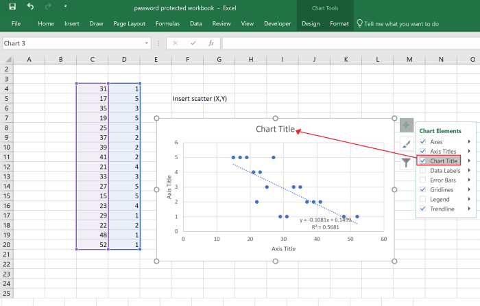
How to Make a Scatter Plot in Excel (Step-By-Step) | Create Scatter ... Go to Design. Click on "Add Chart element". Now, Click on "Trendline". Then, Click on "More trendline options". Click on 'More trend line options', you will see 'Format trendline" on the right side of your excel. Scroll this down to see "Display equation on the chart".

How to Make a Scatter Plot in Excel: Easy Tutorial to | Tripboba.com

How to Create a Scatterplot with Multiple Series in Excel Sep 02, 2021 · Often you may want to create a scatterplot with multiple series in Excel, similar to the plot below: Fortunately this is fairly easy to do in Excel with some simple formulas. The following step-by-step example shows exactly how to do so. Step 1: Enter the Data. First, let’s enter the following (X, Y) values for four different groups: A, B, C ...

Advanced Graphs Using Excel : 3D plots (wireframe, level , contour) in Excel

How To Create A Forest Plot In Microsoft Excel - Top Tip Bio Note, that the study with the smallest Position value will be placed at the bottom of the forest plot. 3. Add a scatter plot to your graph. The next step is to use these new Position values to create a scatter plot, so it looks more like a forest plot. So, right-click on the graph and go to Select Data. Then you want to add a new Series.

How to Create a Scatter Plot in Excel - TurboFuture - Technology

How to Make a Scatter Plot in Excel (XY Chart) - Trump Excel By default, data labels are not visible when you create a scatter plot in Excel. But you can easily add and format these. Do add the data labels to the scatter chart, select the chart, click on the plus icon on the right, and then check the data labels option. This will add the data labels that will show the Y-axis value for each data point in the scatter graph. To format the data labels ...

5 Quick and Easy Data Visualizations in Python with Code

How can I add data labels from a third column to a scatterplot? Under Labels, click Data Labels, and then in the upper part of the list, click the data label type that you want. Under Labels, click Data Labels, and then in the lower part of the list, click where you want the data label to appear. Depending on the chart type, some options may not be available.

How to Create a Scatter Plot in Excel - TurboFuture - Technology

How to Create a Stem-and-Leaf Plot in Excel - Automate Excel You have now gathered all the puzzle pieces needed to create a scatter plot. Let’s put them together. Let’s put them together. Highlight all the values in columns Stem and Leaf Position by selecting the data cells from Column C then holding down the Control key as you select the data cells from Column E, leaving out the header row cells ( C2:C25 and E2:E25 ).

How to Create a Scatter Plot in Excel

Create a Pareto Chart in Excel (In Easy Steps) - Excel Easy 10. Plot the Cumulative % series on the secondary axis. 11. Click OK. Note: Excel 2010 does not offer combo chart as one of the built-in chart types. If you're using Excel 2010, instead of executing steps 8-10, simply select Line with Markers and click OK. Next, right click on the orange/red line and click Format Data Series. Select Secondary ...

Sweetsugarcandies: גרף X Y

How to Add Labels to Scatterplot Points in Excel - Statology Step 3: Add Labels to Points. Next, click anywhere on the chart until a green plus (+) sign appears in the top right corner. Then click Data Labels, then click More Options…. In the Format Data Labels window that appears on the right of the screen, uncheck the box next to Y Value and check the box next to Value From Cells.

31 Label Scatter Plot Excel - Label Design Ideas 2020

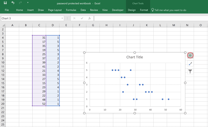
How to Create Scatter Plot In Excel - Career Karma 2. Display the Scatter Chart. Once you have inputted the data, select the desired columns, go to the Insert tab in Excel, select the XY Scatter Chart and choose the first scatter plot option. Now you should have a scatter graph shown in your Excel file. With this done, you need to add a chart title to the scatter plot.

How to Create Scatter Plots in Excel

Scatter plot excel with labels - fmsgyf.stoffwechsel-ev.de So, for the first data set, they tested the cash-out charge. To make a scatter plot , select the data set, go to Recommended Charts from the Insert ribbon and select a Scatter (XY) Plot . Press ok and you will create a scatter plot in excel ..

Plot scatter graph in Excel graph with 3 variables in 2D - Super User

Add Custom Labels to x-y Scatter plot in Excel Step 1: Select the Data, INSERT -> Recommended Charts -> Scatter chart (3 rd chart will be scatter chart) Let the plotted scatter chart be. Step 2: Click the + symbol and add data labels by clicking it as shown below. Step 3: Now we need to add the flavor names to the label. Now right click on the label and click format data labels.

How to Create a Scatter Plot in Excel | TurboFuture

Improve your X Y Scatter Chart with custom data labels - Get Digital Help The first 3 steps tell you how to build a scatter chart. Select cell range B3:C11 Go to tab "Insert" Press with left mouse button on the "scatter" button Press with right mouse button on on a chart dot and press with left mouse button on on "Add Data Labels"

How to Make a Scatter Plot in Excel | Itechguides.com

How to create a scatter plot and customize data labels in Excel During Consulting Projects you will want to use a scatter plot to show potential options. Customizing data labels is not easy so today I will show you how th...

How to Create Scatter Plot in Excel | Excelchat

How to Add Axis Labels in Excel Charts - Step-by-Step (2022) - Spreadsheeto Left-click the Excel chart. 2. Click the plus button in the upper right corner of the chart. 3. Click Axis Titles to put a checkmark in the axis title checkbox. This will display axis titles. 4. Click the added axis title text box to write your axis label. Or you can go to the 'Chart Design' tab, and click the 'Add Chart Element' button ...

Share :